Trying to hide the contents of a cell by simply changing the fill colour of the cell and then matching the font colour so that it blends in perfectly is sometimes an acceptable solution, but you can run into problems when you start highlighting cells or applying conditional formatting. Something like adding in row striping can cause any cell values that you've tried to hide to suddenly be revealed.
Yes, there's a more elegant way to hide the contents of cells. You can do it without messing around with the font and fill colours, and you can do it without hiding entire rows or columns.
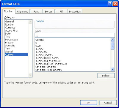
First, select the cell or range of cells that you would like to hide. Right-click and choose 'Format Cells...'. Now, make sure you're in the 'Number' tab of the 'Format Cells' window that pops up. From the list on the left hand side, choose the very last option, 'Custom'. Now, to the right hand side of the window, type in three semicolons in the 'Type' text box. It should look like this:
Click the 'OK' button when you're done, and you'll see all of the values of the cells that you selected will have disappeared.
How does it work?
Custom number formats allow you to choose how you’d like the contents of a cell to be displayed. There are four different sections to a number format: positive numbers, negative numbers, zero values, and finally text values. When you specify a custom number format, you separate these different sections with a semi-colon. I’m not going to go into detail about how to set different number formats in today’s post, but the reason why the values are hidden when you enter ‘;;;’ as a number format is because you’ve told Excel to show nothing for positive numbers, nothing for negative numbers, nothing for zero values, and nothing for text values. The result is a cell that looks completely empty despite containing a value.
Read More
Yes, there's a more elegant way to hide the contents of cells. You can do it without messing around with the font and fill colours, and you can do it without hiding entire rows or columns.
First, select the cell or range of cells that you would like to hide. Right-click and choose 'Format Cells...'. Now, make sure you're in the 'Number' tab of the 'Format Cells' window that pops up. From the list on the left hand side, choose the very last option, 'Custom'. Now, to the right hand side of the window, type in three semicolons in the 'Type' text box. It should look like this:

Click the 'OK' button when you're done, and you'll see all of the values of the cells that you selected will have disappeared.
How does it work?
Custom number formats allow you to choose how you’d like the contents of a cell to be displayed. There are four different sections to a number format: positive numbers, negative numbers, zero values, and finally text values. When you specify a custom number format, you separate these different sections with a semi-colon. I’m not going to go into detail about how to set different number formats in today’s post, but the reason why the values are hidden when you enter ‘;;;’ as a number format is because you’ve told Excel to show nothing for positive numbers, nothing for negative numbers, nothing for zero values, and nothing for text values. The result is a cell that looks completely empty despite containing a value.

